TADs and TAD boundaries
To follow this tutorial, download the FAN-C example data, for example through our
Keeper library. Then run the
example fanc auto command in Example analysis to generate all the
necessary files, and set up your Python session like this:
import fanc
import fanc.plotting as fancplot
import logging

logging.basicConfig(level=logging.INFO, format="%(asctime)s %(levelname)s %(message)s")

hic_100kb = fanc.load("output/hic/binned/fanc_example_100kb.hic")
If you want to try the tutorial with an equivalent Cooler file, load the Hi-C file like this instead:
hic_100kb = fanc.load("architecture/other-hic/fanc_example.mcool@100kb")
or like this if you want to work with a Juicer file built from the same data:
hic_100kb = fanc.load("architecture/other-hic/fanc_example.juicer.hic@100kb")
Note that there may be minor differences in the results due to the “zooming” and balancing applied by the different tools.
Also have a look at the command line documentation at Hi-C domain analysis, which explains a lot of the principles behind insulation scores and directionality indexes with a couple of helpful illustrations.
Insulation scores
Insulation scores are calculated and saved to disk using the InsulationScores
class. To run a basic insulation score calculation on a Hi-C object, use
from_hic:
insulation = fanc.InsulationScores.from_hic(hic_100kb,
                                            [5000000, 1000000, 1500000,
                                             2000000, 2500000, 3000000,
                                             3500000, 4000000],
                                            file_name="architecture/domains/fanc_example_100kb.insulation")
The file created in file_name can later be easily loaded with load().
The resulting object stores all insulation score tracks for the window_sizes
provided. It is derived from the RegionsTable class, which is
RegionBased. There is a lot of convenient functionality
bundled in these objects, which you can read about in RegionBased.
You can access the calculated scores by using the
scores() function, which requires
the window size of the scores you want to retrieve, and returns a list of scores,
one for each genomic region in the object:
scores = insulation.scores(1000000)
However, a more flexible way to retrieve scores, which allows things like subsetting and
retrieving region information at the same time, is the regions()
iterator. Scores are stored as a region attribute insulation_<window size>:
for region in insulation.regions('chr18'):
    score = region.insulation_1000000
    # do something with score
    # ...
If you prefer to have a dedicated object for a particular window size, you can use
score_regions(). The score is then
accessible via the score attribute:
insulation_1mb = insulation.score_regions(1000000)
for r in insulation_1mb.regions:
    score = r.score
Insulation calculation parameters
from_hic has several parameters that
allow you to customise the insulation score calculation. You can read everything them in the
linked API reference, and we will highlight the most important ones here.
impute_missing allows you to replace missing or masked pixels with their expected values
prior to the insulation score calculation. While this avoids dealing with missing pixels,
this can be misleading in case larger regions are unmappable or have been filtered out for
some other reason, so enable this setting with caution. The related parameter
na_threshold instead controls how much of a sliding window can be covered by missing
pixels before assigning it NaN by default. This is set to 0.5 by default - by increasing
this value you will obtain more robust scores, but also the number of NaNs will increase in
your results. Whatever value you choose, it is a tradeoff between information content and
accuracy. In most cases you should be okay with the default setting.
normalise, which is enabled by default, divides insulation scores by their chromosome
mean, so every score is expressed relative to the expected score on the same chromosome. By
disabling this option, you will get raw sums of weights in the sliding window. Normalisation
is stringly recommended, however. You can also normalise to a more local region instead of the
whole chromosome, which may account for local variations in contact intensity other than
insulation. For this purpose, set normalisation_window to a number of bins, for example
300, which is then the number of scores surrounding each region used for normalisation by
their mean.
After their computation and normalisation, insulation scores are log2-transformed. This
makes scores (roughly) symmetrical around 0. To disable this, for example if you have also
disabled normalise, use log=False.
The original insulation score definition uses the arithmetic mean to normalise the scores.
If you expect insulation score outliers in your data, which might affect the normalisation by
the mean, you can use a trimmed arithmetic mean instead by setting trim_mean_proportion
to a value between 0 and 1. The top fraction of insulation scores is then discarded for
calculating the mean.
If you intend to compare scores from different samples (and have the normalise and
log options enabled), a mathematically more accurate normalisation would be to use the
geometric mean instead. You can enable this by setting geometric_mean=True.
Insulation score export
You can export scores to a human-readable file format using one of
to_bed(), or
to_gff(). Export to a fast BigWig track using
to_bigwig().
insulation.to_bed("architecture/domains/fanc_example_100kb.insulation_1mb.bed", 1000000)
Insulation score plots
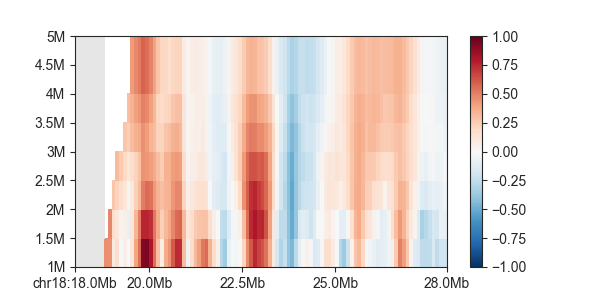
You can plot all calculated insulation scores using GenomicVectorArrayPlot:
p = fancplot.GenomicVectorArrayPlot(insulation, colormap='RdBu_r', vmin=-1, vmax=1,
                                    genomic_format=True)
p.plot('chr18:18mb-28mb')
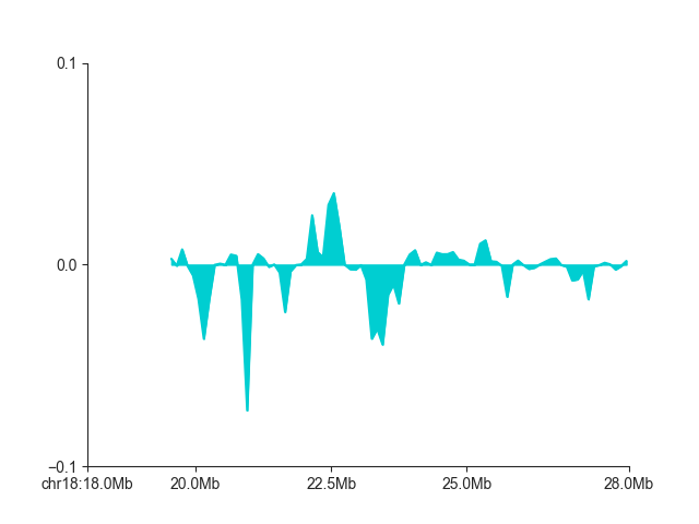
If you only want to plot a single score track, use LinePlot:
p = fancplot.LinePlot(insulation, ylim=(-1, 1), colors=['darkturquoise'], style="mid",
                      attribute="insulation_1000000")
p.plot('chr18:18mb-28mb')
You can read more about different plot types in Plotting (API).
Boundary calls
Once you have the insulation object, you can call insulating boundaries in the genome
using Boundaries, specifically
from_insulation_score():
boundaries = fanc.Boundaries.from_insulation_score(insulation, window_size=1000000)
This finds all minima in the insulation score vector and returns the corresponding regions
as a RegionsTable object, which is RegionBased. The
boundary strength is stored in the score attribute of each region:
for boundary in boundaries.regions:
    score = boundary.score
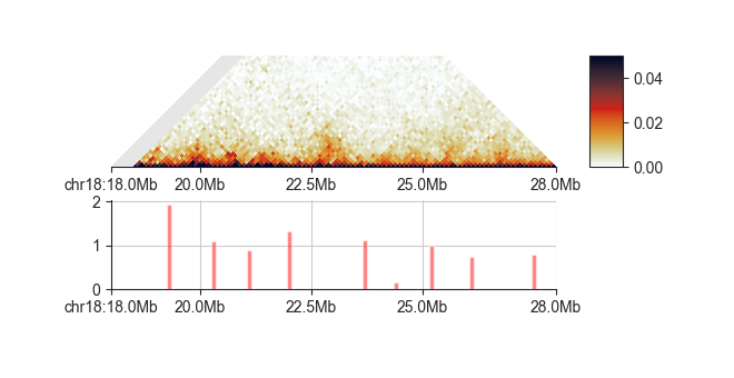
By default, all minima are reported, including very weak and likely false-positive boundaries. We recommend plotting the boundaries and their strength alongside the Hi-C matrix and then decide on a score cutoff to only select a robust set of boundaries!
ph = fancplot.TriangularMatrixPlot(hic_100kb, max_dist=5000000, vmin=0, vmax=0.05)
pb = fancplot.BarPlot(boundaries)
f = fancplot.GenomicFigure([ph, pb])
fig, axes = f.plot('chr18:18mb-28mb')
You can filter out false-positives manually like this
min_score = 1.0
robust_boundaries = []
for boundary in boundaries.regions:
    score = boundary.score
    if score >= min_score:
        robust_boundaries.append(boundary)
or by simply using the min_score argument:
robust_boundaries = fanc.Boundaries.from_insulation_score(insulation, window_size=1000000,
                                                          min_score=1.0)
Directionality index
For a short explanation of the directionality index, please read Directionality Index.
The principle to compute the directionality index is highly similar to the insulation score.
The dedicated class DirectionalityIndexes handles all
relevant actions. Use from_hic() to
compute it for multiple window sizes:
directionality = fanc.DirectionalityIndexes.from_hic(hic_100kb,
                                                     [1000000, 1500000,
                                                      2000000, 2500000, 3000000,
                                                      3500000, 4000000],
                                                     file_name="architecture/domains/fanc_example_100kb.di")
Plotting also works the same way, for all indexes:
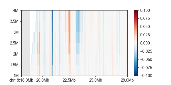
p = fancplot.GenomicVectorArrayPlot(directionality, colormap='RdBu_r', vmin=-0.1, vmax=0.1,
                                    genomic_format=True)
p.plot('chr18:18mb-28mb')
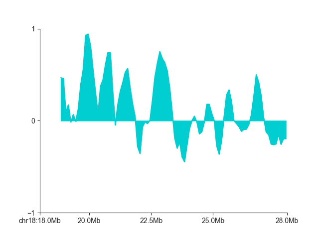
And for single a single directionality index:
p = fancplot.LinePlot(directionality, ylim=(-0.1, 0.1), colors=['darkturquoise'], style="mid",
                      attribute="directionality_4000000")
p.plot('chr18:18mb-28mb')