Loop calling
To follow this tutorial, download the FAN-C example data, for example through our Keeper library, and set up your Python session like this:
import fanc
import fanc.peaks
import fanc.plotting as fancplot

import logging
logging.basicConfig(level=logging.INFO, format="%(asctime)s %(levelname)s %(message)s")

#hic_10kb = fanc.load("architecture/other-hic/bonev2017_esc_10kb.chr1.hic")
hic_sample = fanc.load("architecture/loops/rao2014.chr11_77400000_78600000.hic")
Also have a look at the command line documentation at Loop calling for the command-line approach to loop calling in FAN-C.
Loop calling in FAN-C is a 3-step process:
- Annotate pixels with local enrichment, probability, and mappability information
- Filter pixels based on suitable cutoffs to identify pixels that are part of a loop
- Merge nearby pixels into a single loop call
Annotate pixels
Start by annotating each pixel with loop information using the
RaoPeakCaller and call_peaks() function:
loop_caller = fanc.RaoPeakCaller()
loop_info = loop_caller.call_peaks(hic_sample,
                                   file_name="architecture/loops/rao2014.chr11_77400000_78600000.loop_info")
This creates a RaoPeakInfo object, which contains a bunch of information
on each pixel. Here are the most important ones:
weightanduncorrectedare the normalised and raw contact strength, respectivelye_d,e_h,e_v, ande_llare the expected values calculated from the donut, horizontal, vertical, and lower left neighborhoods, repectively, of the pixeloe_d,oe_h,oe_v,oe_llare the observed/expected (O/E) values calculated from the donut, horizontal, vertical, and lower left neighborhoods, repectively, of the pixelfdr_d,fdr_h,fdr_v,fdr_llare the false discovery rates (FDRs) calculated from the donut, horizontal, vertical, and lower left neighborhoods, repectively, of the pixelmappability_d,mappability_h,mappability_v,mappability_llare the mappabilities of the donut, horizontal, vertical, and lower left neighborhoods, repectively, of the pixel. This is a value between 0 and 1 stating how many pixels in each neighborhood have valid weights
By default, most intra-chromosomal pixels will receive this information, but you have some
influence over the computation with additional parameters. For example, loops tend to occur
away from the diagonal, so you may want to exclude pixels near the diagonal using min_locus_dist,
whihc is expressed in bins. You can also change the values for p and w_init (see original
publication for details) - otherwise sensible defaults are chosen. min_mappable_fraction
controls which pixels are excluded if their local neighbourhoods are below a certain mappability
fraction, which is 0.7 by default, i.e. 70% of each neighbourhood must be valid.
Finally, loops calling is very resource intensive and needs to be heavily parallelised. The number
of parallel processes is controlled with n_processes. By default, this runs loop calling
locally. However, we highly recommend setting cluster=True if you are in a cluster environment
that supports DRMAA (e.g. SGE, Slurm). You may need to set the DRMAA_LIBRARY_PATH environment
variable to the location of your libdrmaa.so in your shell in order for this to work.
call_peaks() must then be called from a head node in order to be
able to submit jobs to the cluster. Read more about the interface with DRMAA in the
gridmap package.
To access the new pixel information, you can use the peaks() iterator:
for edge in loop_info.peaks(lazy=True):
    print(edge.oe_d, edge.fdr_d)
We can also plot it like a regular matrix:
# regular Hi-C
p_hic = fancplot.TriangularMatrixPlot(loop_info, vmin=0, vmax=0.05,
                                      max_dist=600000)
# Donut O/E values
p_oe_d = fancplot.TriangularMatrixPlot(loop_info, vmin=0, vmax=4,
                                       weight_field='oe_d', colormap='Reds',
                                       max_dist=600000)
# Donut FDR values
p_fdr_d = fancplot.TriangularMatrixPlot(loop_info, vmin=0, vmax=0.1,
                                        weight_field='fdr_d', colormap='binary_r',
                                        max_dist=600000)

gf = fancplot.GenomicFigure([p_hic, p_oe_d, p_fdr_d], ticks_last=True)
fig, axes = gf.plot('chr11:77.4mb-78.6mb')
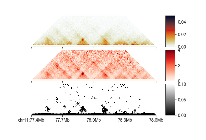
Note how we are controlling which attribute is plotted with weight_field.
These kinds of plots can be extremely useful to choose appropriate filtering thresholds for each of these attributes, which we will see in the next section.
Filter pixels
Based on the annotation, we can try to filter out pixels that are not part of loops. This can be done with filters, specifically
EnrichmentPeakFilterfilters pixels below a minimum O/E in specific neighborhoodsFdrPeakFilterfilters pixels with an FDR higher than specified in each neighborhoodMappabilityPeakFilterfilters pixels with a minimum mappable fraction below the specified cutoffsObservedPeakFilterfilters pixels that do not have a minimum number of raw reads mapping to themDistancePeakFilterfilters pixels that are closer than a certain number of bins from the diagonal
Each of these is instantiated and then added to the object using
filter(). When applying multiple filters it is recommended to
first queue them using queue=True and to run all of them together with
run_queued_filters():
# filter on O/E
enrichment_filter = fanc.peaks.EnrichmentPeakFilter(
        enrichment_ll_cutoff=1.75,
        enrichment_d_cutoff=3,
        enrichment_h_cutoff=2,
        enrichment_v_cutoff=2)
loop_info.filter(enrichment_filter, queue=True)

# filter on FDR
fdr_filter = fanc.peaks.FdrPeakFilter(
    fdr_ll_cutoff=0.05,
    fdr_d_cutoff=0.05,
    fdr_h_cutoff=0.05,
    fdr_v_cutoff=0.05)
loop_info.filter(fdr_filter, queue=True)

# filter on mappability
mappability_filter = fanc.peaks.MappabilityPeakFilter(
    mappability_ll_cutoff=0.7,
    mappability_d_cutoff=0.7,
    mappability_h_cutoff=0.7,
    mappability_v_cutoff=0.7)
loop_info.filter(mappability_filter, queue=True)

# filter on distance from diagonal
distance_filter = fanc.peaks.DistancePeakFilter(5)
loop_info.filter(distance_filter, queue=True)

# filter on minimum number of observed values
observed_filter = fanc.peaks.ObservedPeakFilter(10)
loop_info.filter(observed_filter, queue=True)

loop_info.run_queued_filters()
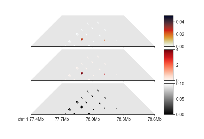
We could also tweak the above cutoffs to further remove noisy pixels. The next step is to merge pixels belonging to the same loop into loop calls.
Merge pixels
To merge the remaining pixels into loops use
merged_peaks = loop_info.merged_peaks()
merged_peaks now contains putative loop calls. However, there will still be a number of
false-positive loops in this object, which typically consist of a single enriched pixel, likely
due to noise. Real loops generally consist of multiple pixels. We can remove the “singlets”
using RaoMergedPeakFilter:
singlet_filter = fanc.peaks.RaoMergedPeakFilter(cutoff=-1)
merged_peaks.filter(singlet_filter)
A cutoff here of -1 remove all singlets. In Rao, Huntley et al. (2014) they only remove
singlets if their qvalue sum is larger than 0.02, which you can use instead of -1
and particularly strong singlets will still be kept in the data.
For our example dataset this leaves only a single loop, which we can export with
to_bedpe():
# regular Hi-C
merged_peaks.to_bedpe("architecture/loops/rao2014.chr11_77400000_78600000.bedpe")
# chr11	77807143	77842857	chr11	77947143	77982857	.	0.0