Aggregate analyses
To follow this tutorial, download the FAN-C example data, for example through our
Keeper library. Then run the
example fanc auto command in Example analysis to generate all the
necessary files, and set up your Python session like this:
import fanc
import fanc.plotting as fancplot

import logging
logging.basicConfig(level=logging.INFO, format="%(asctime)s %(levelname)s %(message)s")

hic_100kb = fanc.load("output/hic/binned/fanc_example_100kb.hic")
hic_rao = fanc.load("architecture/loops/rao2014.chr11_77400000_78600000.hic")

boundaries = fanc.load("architecture/domains/fanc_example_100kb.insulation_boundaries_score_0.7_1mb.bed")
tads = fanc.load("architecture/domains/gm12878_tads.bed")
loops = fanc.load("architecture/loops/rao2014.chr11_77400000_78600000.loops_no_singlets.bedpe")
If you want to try the tutorial with an equivalent Cooler file, load the Hi-C file like this instead:
hic_100kb = fanc.load("architecture/other-hic/fanc_example.mcool@100kb")
or like this if you want to work with a Juicer file built from the same data:
hic_100kb = fanc.load("architecture/other-hic/fanc_example.juicer.hic@100kb")
Note that there may be minor differences in the results due to the “zooming” and balancing applied by the different tools.
Also have a look at the command line documentation at Hi-C aggregate analysis, which explains the different types of aggregate analyses with helpful illustrations.
Aggregate analyses can provide a general overview of the 3D genomic structure around a set of interesting genomic regions. This is achieved by aggregating, i.e. averaging, the matrices around each region to obtain a single, aggregated view of all regions at the same time.
FAN-C distinguished three kinds of aggregate analyses:
- Fixed-size regions along the matrix diagonal, for example a window of 500kb around each active TSS in the genome
- Variable-size regions along the matrix diagonal, for example TADs in the genome or genes from 5’ to 3’
- Region pairs, denoting a part of the matrix off the diagonal, for example loops in the Hi-C matrix
All of these can be computed using the AggregateMatrix
class, and dedicated functions for each analysis type.
Fixed-size regions
Fixed-size analyses are the simplest aggregate analyses. All you need is a list of regions
of interest, for example insulating boundaries, and they can be computed using
from_center() like this:
fixed_am = fanc.AggregateMatrix.from_center(hic_100kb, boundaries.regions,
                                            window=5000000)
You can optionally supply a file_name to save the aggregate matrix and all its components
to disk.
The window parameter is crucial here and sets the window around the center of each region
that should be extracted. If the window lies outside the chromosome boundaries, the region is
declared as “invalid” and not used for the aggregate matrix. Despite being named from_center,
it is possible to use another point in each region as relative window center with region_viewpoint.
You can set this to any of start, end, five-prime, and three_prime and the window
will be centred on that part of each region. For example, use five_prime to aggregate the
region around the TSS’s in a list of genes.
You can plot the aggregate matrix using the covenience function aggregate_plot():
ax = fancplot.aggregate_plot(fixed_am, vmin=-1, vmax=1,
                             labels=['-2.5Mb', 'boundary', '+2.5Mb'])
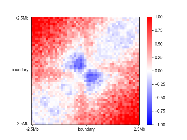
In this case you can nicely see the boundary in the centre of the plot. By default, an aggregate
analysis always uses O/E transformed matrices, as otherwise the distance decay might bias the result
too much, particular for a chromosome-based normalisation strategy, as is the default in FAN-C.
You can switch this off using oe=False, however.
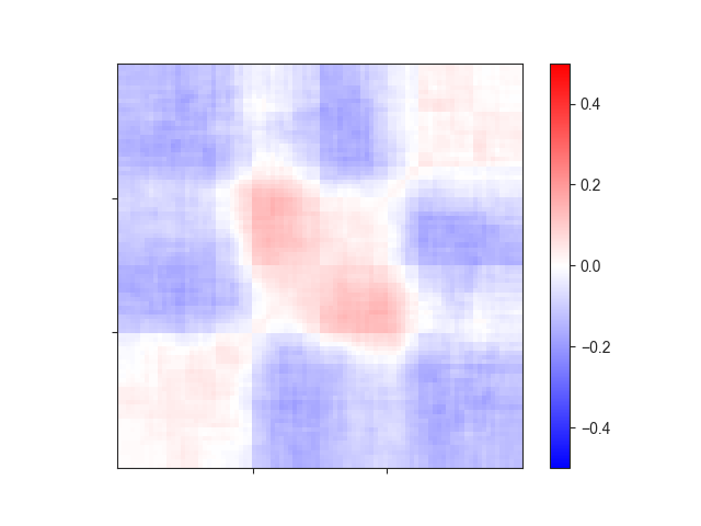
Variable-size regions
The command for variable-size regions such as TADs is highly similar:
variable_am = fanc.AggregateMatrix.from_regions(hic_100kb, tads.regions)
By default, each region is extended by each own length on each side (relative_extension=1.0),
which is a useful preset for TADs so that the regions are clearly visible in the centre.
We can visualise the region using aggregate_plot()
ax = fancplot.aggregate_plot(variable_am, vmin=-0.5, vmax=0.5,
                             relative_label_locations=[0.33, 0.66])
To generate an aggregate matrix from variable-size regions, the extracted matrices first have to be
extrapolated to the same size. This is done internally using resize() from
the skimage.transform module. You can determine the type of interpolation using the
interpolation argument, which is an integer: 0: Nearest-neighbor (default), 1: Bi-linear,
2: Bi-quadratic, 3: Bi-cubic, 4: Bi-quartic, 5: Bi-quintic. You can also turn off antialiasing
in case you feel that this is a source of bias.
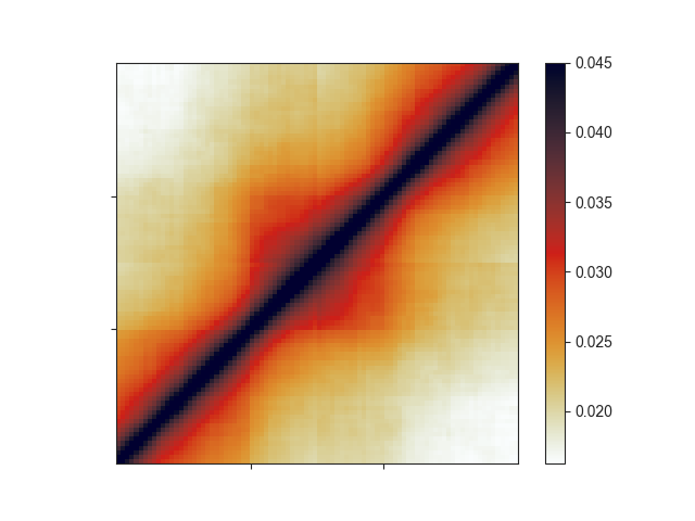
For TADs or other regions along the diagonal specifically, you can also rescale the aggregate
matrix, which applies an artificial exponential decay to the matrix, making it resemble a Hi-C
matrix:
rescale_am = fanc.AggregateMatrix.from_regions(hic_100kb, tads.regions,
                                               rescale=True, log=False)
ax = fancplot.aggregate_plot(rescale_am, vmax=0.045,
                             relative_label_locations=[0.33, 0.66],
                             colormap='germany')
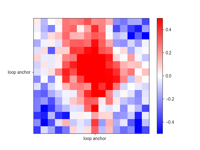
Region pairs
So far, we have only aggregated regions along the diagonal.
from_region_pairs() allows us to aggregate
arbitrary region pairs, albeit without extrapolation of differently-sized regions - only fixed
window sizes are supported. You can either supply a window, as with fixed-size regions
along the diagonal, or a number of pixels/bins, which is set to 16 by default.
Here is an example for loops:
loops_am = fanc.AggregateMatrix.from_center_pairs(hic_rao, loops.region_pairs())
ax = fancplot.aggregate_plot(loops_am, vmin=-0.5, vmax=0.5,
                             relative_label_locations=[0.5],
                             labels=['loop anchor'])
Useful functions
If you don’t just want to plot the aggregate matrix, but work with its values, you can access
it as a numpy array via matrix():
m = fixed_am.matrix()
type(m)  # numpy.ndarray
All aggregate functions discussed above have a keep_components parameter, which is True
by default. This way, all the matrix that have been extracted from regions or region pairs are
stored inside the aggregate matrix object. You can access them via
components():
for component_matrix in fixed_am.components():
    shape = component_matrix.shape  # 51, 51
    # ...
These individual matrices can be very useful to debug a troublesome aggregate plot, because often
it is unusual outlier matrices that have a large effect on the plot. They are simply numpy
arrays, which you can plot with imshow from matplotlib, for example.