PCA
To follow this tutorial, download the FAN-C example data, for example through our Keeper library. Then set up your Python session like this, loading some of our previously published Low-C datasets:
import fanc
import fanc.plotting as fancplot
from fanc.architecture.comparisons import hic_pca

lowc_hindiii_100k = fanc.load("architecture/other-hic/lowc_hindiii_100k_1mb.hic")
lowc_hindiii_5M = fanc.load("architecture/other-hic/lowc_hindiii_5M_1mb.hic")
lowc_mboi_1M = fanc.load("architecture/other-hic/lowc_mboi_1M_1mb.hic")
lowc_mboi_100k = fanc.load("architecture/other-hic/lowc_mboi_100k_1mb.hic")
lowc_mboi_50k = fanc.load("architecture/other-hic/lowc_mboi_50k_1mb.hic")
PCA is one way in FAN-C to compare different Hi-C matrices to each other. A matrix of pixels vs matrices is assembled that contains the (normalised) contact strength of each matrix for the respective pixel (=region pair). PCA is then run on this matrix, and the resulting eigenvectors can be plotted to examine the variability between datasets.
In FAN-C, simply use hic_pca() for this purpose,
as shown here for chromosome 19:
pca_info, pca_result = hic_pca(lowc_hindiii_5M, lowc_hindiii_100k,
                               lowc_mboi_1M, lowc_mboi_50k,
                               lowc_mboi_100k, ignore_zeros=True,
                               scale=False, region='chr19', sample_size=100000,
                               strategy='variance')
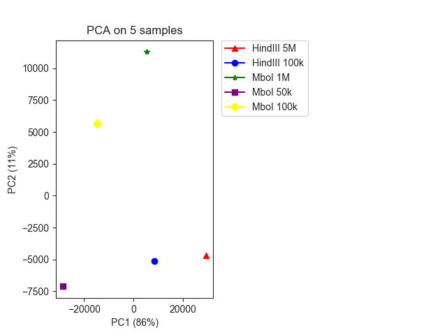
We can plot the result using pca_plot():
fig, ax = fancplot.pca_plot(pca_result, variance=pca_info,
                            names=["HindIII 5M", "HindIII 100k",
                                   "MboI 1M", "MboI 50k", "MboI 100k"])
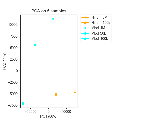
We can easily change the colors and markers, for example by colouring all samples with MboI and HindIII differently, and assigning different markers to samples with more or less than 1M cells:
fig, ax = fancplot.pca_plot(pca_result, variance=pca_info,
                            names=["HindIII 5M", "HindIII 100k",
                                   "MboI 1M", "MboI 50k", "MboI 100k"],
                            colors=["orange", "orange", "cyan", "cyan", "cyan"],
                            markers=["*", "o", "*", "o", "o"])
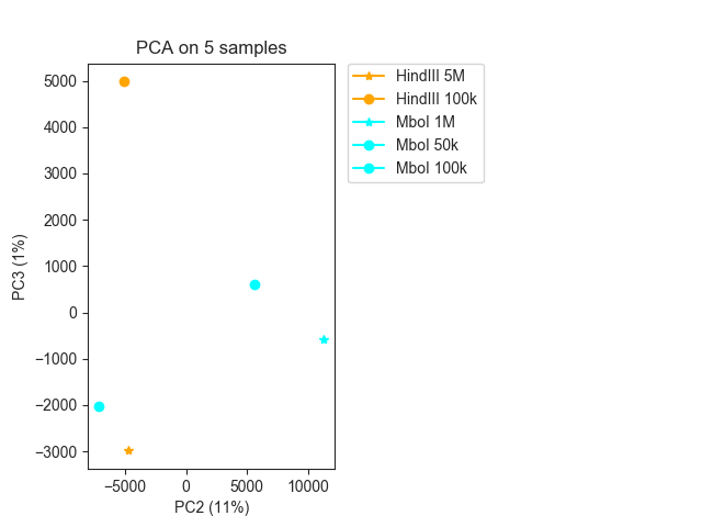
Sometimes the first eigenvector captures the library sequencing depth, so you may want to
plot the second and third EVs instead using eigenvectors=(1,2) (in this case it does
not seem to be particularly informative):
fig, ax = fancplot.pca_plot(pca_result, variance=pca_info,
                            eigenvectors=(1, 2),
                            names=["HindIII 5M", "HindIII 100k",
                                   "MboI 1M", "MboI 50k", "MboI 100k"],
                            colors=["orange", "orange", "cyan", "cyan", "cyan"],
                            markers=["*", "o", "*", "o", "o"])
This kind of analysis can be tricky, and selecting informative pixels from the matrix can
be key to getting a robust and intuitive PCA result. In the above example, we are using
several parameters to select informative pixels for the PCA. First, we are only using
pixels that are non-zero in all samples with ignore_zeros=True. Second, we are sorting
the pixels, listing the ones with the largest variance across samples first, using
strategy='variance'. Finally, we are selecting the top 100k pixels (those with the
largest variance) first with sample_size=100000.
When you are analysing matrices of higher resolution, pixels far away from the diagonal
might be dominated by noise. ignore_zeros removes most of the noisy pixels, but
additionally you might want to set a max_distance to only select pixels corresponding
to regions closer than this value. Similarly, if you want to exclude contacts close to
the diagonal, use min_distance.
For more options have a look at the API reference for pca_plot().