Hi-C aggregate analysis

Note

The following examples use the matrix files in FAN-C format. If you want to try the same commands using Juicer .hic files, replace output/hic/binned/fanc_example_100kb.hic with architecture/other-hic/fanc_example.juicer.hic@100kb. If you want to work with Cooler files in this tutorial, use architecture/other-hic/fanc_example.mcool@100kb. The results will be minimally different due to the “zooming” and balancing applied by each package.

It can be very informative to view the average Hi-C matrix for a set of regions, rather than the Hi-C matrix at each individual region. This can help you in identifying common structural features of these regions or over-/under-representation of contacts in the vicinity.

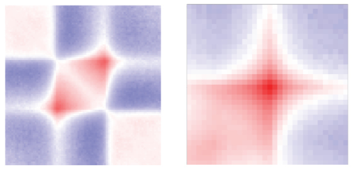
Here are examples of TAD and loop aggregate plots from our recent preprint (Kruse et al. (2019)):

You can easily create your own aggregate plots using fanc aggregate.

usage: fanc aggregate [-h] [-m MATRIX_FILE] [-p PLOT_FILE] [--tads]
                      [--tads-imakaev] [--loops]
                      [--loop-strength LOOP_STRENGTH_FILE]
                      [--tad-strength TAD_STRENGTH_FILE] [-w WINDOW]
                      [--pixels PIXELS] [-v REGION_VIEWPOINT]
                      [-b BOUNDARY_MODE] [-i INTERPOLATION] [-r RELATIVE]
                      [-a ABSOLUTE] [-e] [-l] [--rescale]
                      [--colormap COLORMAP] [--vmin VMIN] [--vmax VMAX] [-tmp]
                      [-C] [--keep-submatrices] [-s] [--lower-triangular-plot]
                      [--labels LABELS] [--label-locations LABEL_LOCATIONS]
                      input [regions] [output]

Positional Arguments

input	FAN-C matrix file (e.g. Hic)
regions	File with regions (BED, GFF, Tabix, …) or region pairs (BEDPE)
output	Output AggregateMatrix file for further processing.See -p and -m option for aggregate plot and matrix, respectively.

Named Arguments

-m, --save-matrix
	Path to save aggregate matrix (numpy txt format)
-p, --save-plot
	Path to save aggregate plot (PDF)
--tads	Use presets for aggregate TADs: –relative 1.0 –expected –log –vmin -1 –vmax 1
--tads-imakaev	Use presets for aggregate TADs: –relative 1.0 –expected–rescale
--loops	Use presets for aggregate loops: –pixels 16 -l
--loop-strength
	Calculate loop strengths and save to file. Only works when providing BEDPE file, and Hi-C matrix.
--tad-strength	Calculate tad strengths and save to file. Only works with –tads preset
-w, --window	Width of the region window used for aggregation. If set, will only use the center position from the input regions and extract a submatrix of width -w around this region.
--pixels	Width of the output image in pixels. Default: 90
-v, --region-viewpoint
	Viewpoint relative to region when using -w. By default, this measures the window from the region center. You can change this to other locations within each region using this parameter. Possible values:start, end, five_prime, three_prime, center
-b, --boundary-mode
	Points outside the boundaries of the input are filled according to the given mode. Options areconstant, edge, symmetrix, reflect, and warp.Default: reflect.
-i, --interpolation
	Type of interpolation to use for resizing. 0: Nearest-neighbor (default), 1: Bi-linear, 2: Bi-quadratic, 3: Bi-cubic, 4: Bi-quartic, 5: Bi-quintic
-r, --relative	Relative extension of each region as fraction of region length (l). Final region in the image will be: <start of region - e*l> to <end of region + e*l>. Default: 1.0 (results in 3 times region size image). Additive with “-a” parameter!
-a, --absolute	Extension (e) of each region in base pairs. Final region in the image will be: <start of TAD - e> to <end of TAD + e>. Default: 0 (no extension). Additive with “-r” parameter!
-e, --expected-norm
	Normalize matrix to expected values
-l, --log	log2-transform normalized matrices. Only used in conjunction with “-e”.
--rescale	Rescale normalized contact matrices using an a=-0.25 power law. Only used in conjunction with “-e”.
--colormap	Matplotlib colormap to use for matrix
--vmin	Minimum saturation value in image
--vmax	Maximum saturation value in image
-tmp, --work-in-tmp
	Work in temporary directory
-C, --no-cache	Do not cache chromosome matrices. Slower, but saves a lot of memory. Use this if you are having trouble with memory usage.
--keep-submatrices
	Save all the individual matrices that make up the aggregate matrix in the output object. Useful for debugging and downstream processing. Potentially uses a lot of memory and/or disk space.
-s, --orient-by-strand
	Flip submatrix if region is on the negative strand.
--lower-triangular-plot
	Invert the aggregate plot so it corresponds to the lower triangle of the Hi-C matrix.
--labels	Labels for the left, center, and right edge of the matrix (comma-separated).
--label-locations
	Relative location of ticks on bottom and left of aggregate plot (comma-separated). Ranges from 0 (left/bottom) to 1.0 (right/top). Default: 0,0.5,1.0

You can provide fanc aggregate with a list of genomic regions in any of the common region-based formats (BED, GFF, BigWig, …) or with a list of genomic region pairs in BEDPE format. For lists of regions, the aggregate matrix will be located at the Hi-C matrix diagonal. For pairs of regions, matrix subsets can be anywhere in the genome.

Aggregate over variable size regions

By default, if you provide fanc aggregate with a list of regions, it will extract the square Hi-C sub-matrices along the diagonal for each region and interpolate them to match the width set by --pixels (90 by default). It will then calculate the average value for each pixel, which then form the aggregate matrix.

Let’s try this on TADs called using the arrowhead algorithm (Rao and Huntley et al., 2014). fanc aggregate will ignore all regions in the file that are not present in the Hi-C matrix. In our example Hic file, that is everything outside of chromosomes 18 and 19:

fanc aggregate output/hic/binned/fanc_example_100kb.hic \
               architecture/domains/gm12878_tads.bed \
               architecture/aggregate/fanc_example_100kb.agg

This command only produces an AggregateMatrix file (fanc_example_100kb.agg), which is useful for further usage with FAN-C, but not easily readable. To extract the aggregate matrix in txt format, simply add -m and to plot it just use -p:

fanc aggregate output/hic/binned/fanc_example_100kb.hic \
               architecture/domains/gm12878_tads.bed \
               architecture/aggregate/fanc_example_100kb.agg \
               -p architecture/aggregate/fanc_example_100kb.agg.png \
               -m architecture/aggregate/fanc_example_100kb.agg.txt

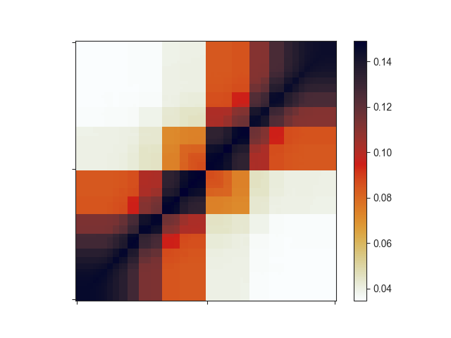
The resulting plot looks a bit strange:

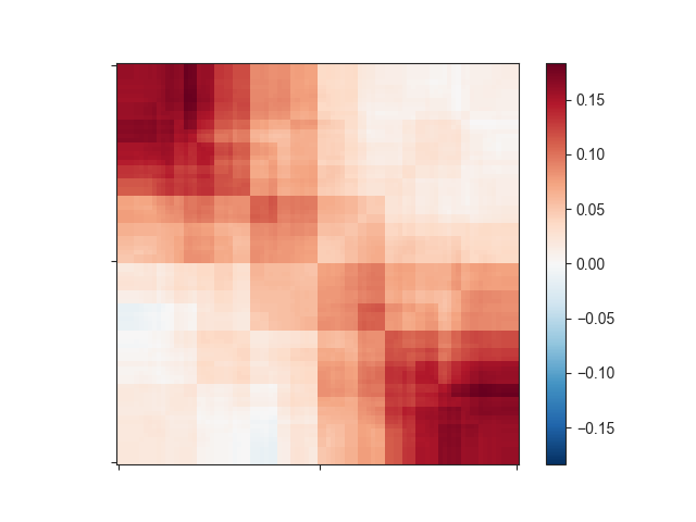
Important note: if your input regions have variable sizes, as assumed in this section, the resulting aggregate matrix with default settings is highly misleading, since smaller regions will have larger average signal in the interpolated matrix due to being closer to the diagonal. You can easily correct for this effect using O/E matrices instead of the regular Hi-C matrix. Simply set the -e flag for this. -e works very well with log2-transformed data (-l). Let’s see how this changes your matrix:

fanc aggregate output/hic/binned/fanc_example_100kb.hic \
               architecture/domains/gm12878_tads.bed \
               architecture/aggregate/fanc_example_100kb.agg \
               -p architecture/aggregate/fanc_example_100kb_oe.agg.png \
               -m architecture/aggregate/fanc_example_100kb_oe.agg.txt \
               -e -l

This still does not look like much of a TAD, but we can add a little more context by expanding the plotting region relative to the region size using -r:

fanc aggregate output/hic/binned/fanc_example_100kb.hic \
               architecture/domains/gm12878_tads.bed \
               architecture/aggregate/fanc_example_100kb.agg \
               -p architecture/aggregate/fanc_example_100kb_oe_large.agg.png \
               -m architecture/aggregate/fanc_example_100kb_oe_large.agg.txt \
               -e -l -r 1.0

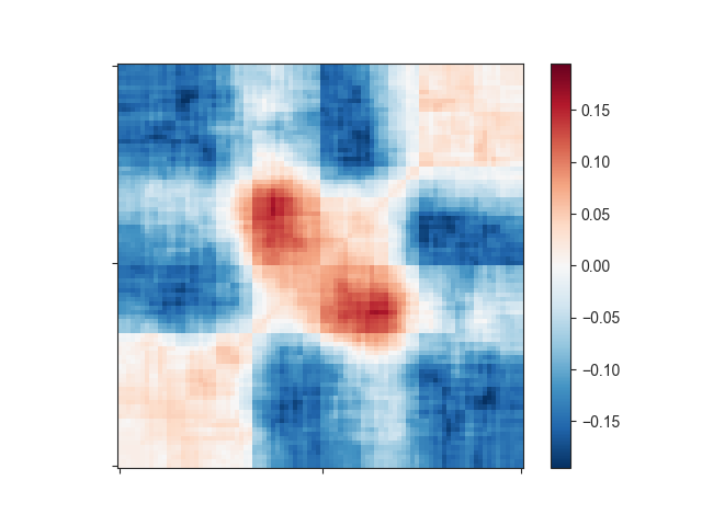
That plot depicts a region that is 3x the size of the TAD located in its center and already looks like we would expect: High signal in the center, especially at the TAD corner, where the corner loops are typically located.

We can further apply an exponential rescaling (--rescale) of the data to make this look more like a Hi-C matrix:

fanc aggregate output/hic/binned/fanc_example_100kb.hic \
               architecture/domains/gm12878_tads.bed \
               architecture/aggregate/fanc_example_100kb.agg \
               -p architecture/aggregate/fanc_example_100kb_oe_large_res.png \
               -m architecture/aggregate/fanc_example_100kb_oe_large.agg.txt \
               -e -r 1.0 --rescale --vmax 0.045

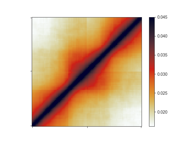
Here, we are not log-transforming the data and we are setting the saturation of the pixel values at 0.045 using --vmax.

Aggregate TADs

For both the log2(O/E) and rescaled versions of the aggregate matrices, there are preset flags you can use called --tads and --tads-imakaev, respectively. The latter is named after the first author of the publication that first used rescaled aggregate matrices in this fashion (Flyamer, Gassler, and Imakaev et al., 2017). In the above example, you can simply run

fanc aggregate output/hic/binned/fanc_example_100kb.hic \
               architecture/domains/gm12878_tads.bed \
               architecture/aggregate/fanc_example_100kb.agg \
               -p architecture/aggregate/fanc_example_100kb_oe_large.agg.png \
               -m architecture/aggregate/fanc_example_100kb_oe_large.agg.txt \
               --tads

Fixed-width regions

Sometimes, you may want to use a fixed window surrounding a set of features in the aggregate analysis, such as TAD boundaries. fanc aggregate provides the -w option to plot the aggregate Hi-C matrix in a window os size w around the center of each region in the list provided.

fanc aggregate output/hic/binned/fanc_example_100kb.hic \
               architecture/domains/fanc_example_100kb.insulation_boundaries_score0.7_1mb.bed \
               architecture/aggregate/fanc_example_100kb_boundaries.agg \
               -w 5mb -p architecture/aggregate/fanc_example_100kb_boundaries.agg.png \
               -m architecture/aggregate/fanc_example_100kb_boundaries.agg.txt \
               --vmin 0 --vmax 0.03

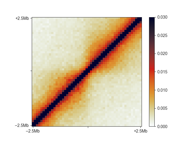
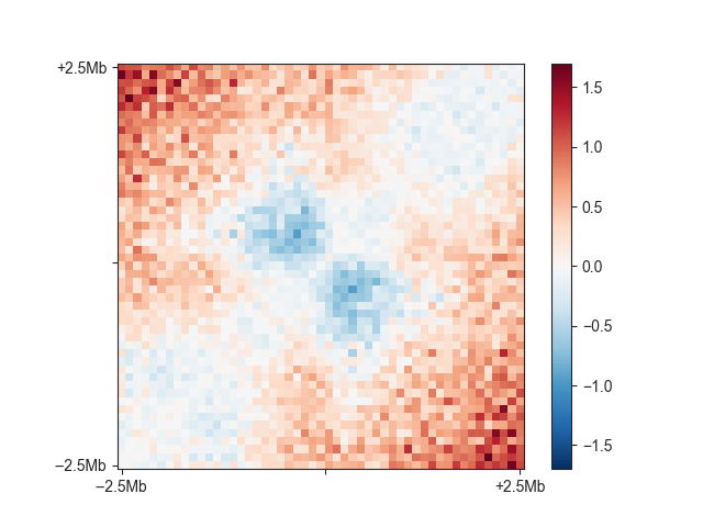
You can see the relatively faint “average boundary” in the centre of the plot. When using O/E and log2-transformed matrices, this becomes much more obvious:

fanc aggregate output/hic/binned/fanc_example_100kb.hic \
               architecture/domains/fanc_example_100kb.insulation_boundaries_score0.7_1mb.bed \
               architecture/aggregate/fanc_example_100kb_boundaries_oe.agg \
               -w 5mb -p architecture/aggregate/fanc_example_100kb_boundaries_oe.agg.png \
               -m architecture/aggregate/fanc_example_100kb_boundaries_oe.agg.txt \
               -e -l

You can change the viewpoint to other positions within a region, such as the 5’ end, using the -v option.

Loops and other pairwise genomic regions

When you have loop calls or other pairwise genomic regions in BEDPE format, you can use fanc aggregate to make aggregate loop plots. The preset for this is --loops.

fanc aggregate architecture/loops/rao2014.chr11_77400000_78600000.hic \
               architecture/loops/rao2014.chr11_77400000_78600000.loops_no_singlets.bedpe \
               architecture/loops/rao2014.chr11_77400000_78600000.loops_no_singlets.agg \
               -p architecture/aggregate/rao2014.chr11_77400000_78600000.loops_no_singlets.agg.png \
               --loops

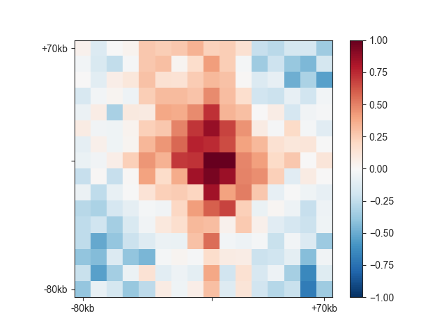
Control the size of the plot using the --pixels argument.