Region and Score panel types
This section will introduce the panel types for region-based data, such as genomic feature definitions or score tracks.
line
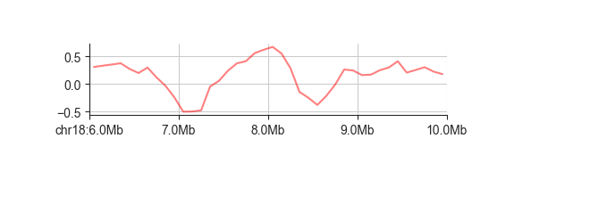
To visualise a single track of continuous scores, a simple line plot generally works very
well. This plot works on any file compatible with the RegionBased interface, which
includes most of the common genomic data containers (BED, GFF, BigWig, Tabix, …) and almost
all FAN-C objects.
fancplot chr18:6mb-10mb -p line architecture/domains/fanc_example_100kb.insulation_1mb.bw
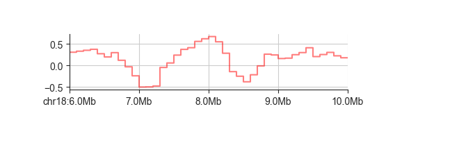
When dealing with regions of variable size or if you want to emphasise that a value is assigned
to an interval rather than a single point, you can change the line style to a stepwise
representation using -s step:
fancplot chr18:6mb-10mb -p line -s step architecture/domains/fanc_example_100kb.insulation_1mb.bw
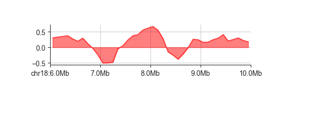
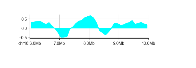
If you like, you can also fill the area between the horizontal line at 0 and the curve
using -f
fancplot chr18:6mb-10mb -p line -f architecture/domains/fanc_example_100kb.insulation_1mb.bw
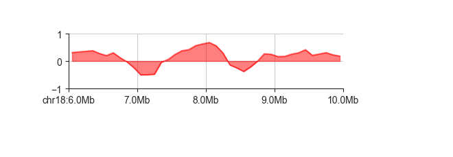
Use -y to set the y axis limits
fancplot chr18:6mb-10mb -p line -f -y -1 1 architecture/domains/fanc_example_100kb.insulation_1mb.bw
You can control color and transparency of the line and its fill with -c and --alpha,
respectively. By default, the alpha value is at 0.5. Any custom value must be between
0 and 1. To make the colors fully opaque, for example, use:
fancplot chr18:6mb-10mb -p line -f -c cyan --alpha 1. architecture/domains/fanc_example_100kb.insulation_1mb.bw
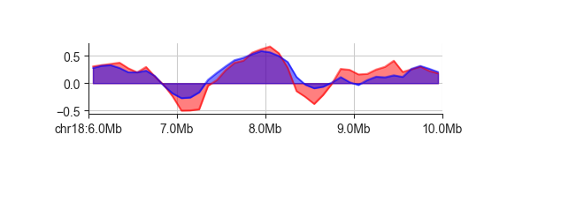
Transparency is especially useful when plotting multiple tracks in the same panels. You can do this by simply adding more datasets.
fancplot chr18:6mb-10mb -p line -f architecture/domains/fanc_example_100kb.insulation_1mb.bw architecture/domains/fanc_example_100kb.insulation_2mb.bw
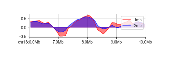
You can label datasets with -l, which will add a legend to your plot. By default,
FAN-C will try to find a placement with minimum overlap to the plotted lines. If you prefer,
you can position the legend somewhere else using the --legend-location parameter.
Possible locations can be found
here.
fancplot chr18:6mb-10mb -p line -l 1mb 2mb -f architecture/domains/fanc_example_100kb.insulation_1mb.bw architecture/domains/fanc_example_100kb.insulation_2mb.bw
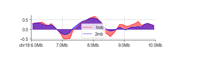
fancplot chr18:6mb-10mb -p line -l 1mb 2mb -f architecture/domains/fanc_example_100kb.insulation_1mb.bw architecture/domains/fanc_example_100kb.insulation_2mb.bw
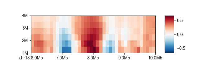
scores
The scores panel type is designed for genome-wide, region-based scores, such as
the insulation score, that depend on a central parameter, such as a window size. It
represents scores in a heatmap, where each line corresponds to a different parameter
value, which allows a quick survey of scores without having to commit to a specific
parameter choice. It currently supports the InsulationScores
and DirectionalityIndexes objects, but can in
principle be extended to other data containers.
fancplot chr18:6mb-10mb -p scores architecture/domains/fanc_example_100kb.insulation

When your parameter represents a measure of base pairs, you can use the --genomic-format
or -g parameter for a more abbreviated representation:
fancplot chr18:6mb-10mb -p scores -g architecture/domains/fanc_example_100kb.insulation
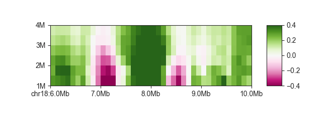
As with regular matrix plots, you can control various plot parameters such as heatmap color and saturation limits:
fancplot chr18:6mb-10mb -p scores -g -c PiYG -vmin -0.4 -vmax 0.4 architecture/domains/fanc_example_100kb.insulation
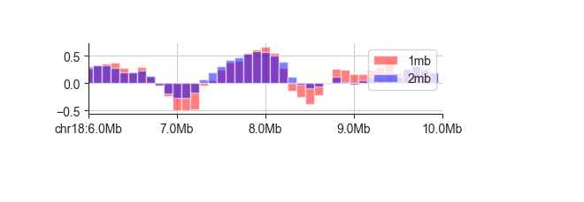
bar
The bar plot can be used almost in exactly the same way as the line plot above, so we
recommend you read about line first. Here is an example:
fancplot chr18:6mb-10mb -p bar -l 1mb 2mb architecture/domains/fanc_example_100kb.insulation_1mb.bw architecture/domains/fanc_example_100kb.insulation_2mb.bw
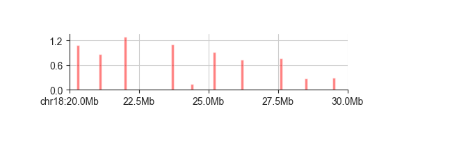
However, bar may be most useful when dealing with sparse data that does not cover every
genomic interval. One example are domain boundaries. Here is a larger region of chr18
showing all possible domain boundaries called from the insulation score (fanc boundaries).
The bar height corresponds to the boundary score:
fancplot chr18:20mb-30mb -p bar architecture/domains/fanc_example_100kb.insulation_boundaries_1mb.bed
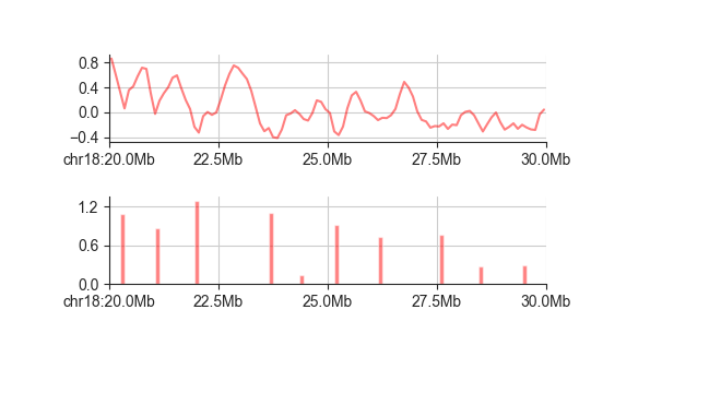
This is especially useful in combination with the line plot of the insulation score, where
you can see exactly that each score minimum corresponds to a boundary call.:
fancplot chr18:20mb-30mb -p line architecture/domains/fanc_example_100kb.insulation_1mb.bw -p bar architecture/domains/fanc_example_100kb.insulation_boundaries_1mb.bed
layer
When you have a set of feature locations without an associated score, you can use a layer
panel to visualise them (this also works for feature with scores, but they will be ignored).
Using the boundary locations above:
fancplot chr18:20mb-30mb -p layer architecture/domains/fanc_example_100kb.insulation_boundaries_1mb.bed
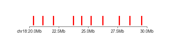
As you can see, this will only plot the location of the provided features as rectangles - the
height is simply a consequence of the panel height and has no biological meaning. (Remember that
you can control the plot height using the --aspect-ratio argument).
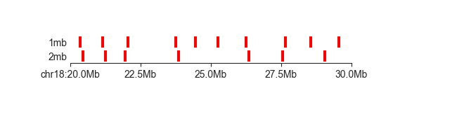
Where the layer plot really shines, and where it gets its name from, is when dealing with
different feature types simultaneously. As an example, we have created a BED file that contains
both the domain boundaries called with a 1mb and a 2mb insulation score window. The 1mb boundaries
have 1mb in the BED “name” field, while the 2mb boundaries appropriately have 2mb. The
name field is used by layer to divide features into rows:
fancplot chr18:20mb-30mb -p layer architecture/domains/fanc_example_100kb.insulation_boundaries_1mb_and_2mb.bed
gene
The feature plot is very versatile, but it cannot handle exon specifications and does not label
individual features. For that purpose, fancplot proves the gene panel. It is intended for use
with GFF files, such as can be obtained from Gencode, although it is in principle compatible with
any RegionBased file (not fully tested). It is most efficient when the GFF files have been sorted
by chromosome and start coordinate, bgzipped and indexed with Tabix
(here is an example you can use for Tabix indexing)