Matrix panel types
This section will provide details about the different types of panels in the
command-line interface of fancplot.
triangular
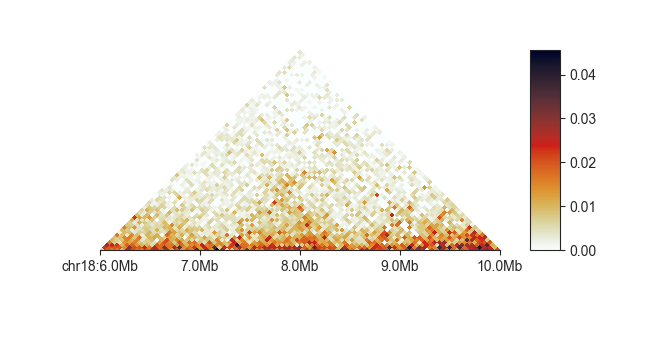
This is the common triangular heatmap plot used primarily for Hi-C data, but which is compatible with all sort of input matrices, including difference and fold-change comparisons. You simply provide it with a FAN-C compatible matrix file:
fancplot chr18:6mb-10mb -p triangular output/hic/binned/fanc_example_50kb.hic
You often need to adjust the matrix saturation, to highlight different parts of the image.
You can do this interactively with -r:
fancplot chr18:6mb-10mb -p triangular -r output/hic/binned/fanc_example_50kb.hic
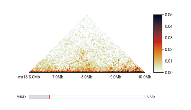
Or by explicitly setting a maximum saturation using -vmax, in this case to 0.05.
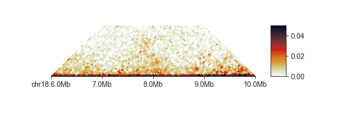
You can truncate the triangle at a certain distance with -m for more compact plots:
fancplot chr18:6mb-10mb -p triangular -m 2mb -vmax 0.05 output/hic/binned/fanc_example_50kb.hic
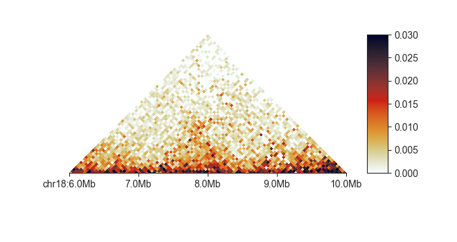
You can also set the lower saturation values directly using -vmin:
fancplot chr18:6mb-10mb -p triangular -vmin 0 -vmax 0.03 output/hic/binned/fanc_example_50kb.hic
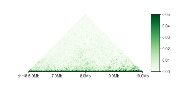
To change the default colormap use -c <matplotlib colormap> - any
colormap in matplotlib
is supported.
fancplot chr18:6mb-10mb -p triangular -c Greens -vmax 0.05 output/hic/binned/fanc_example_50kb.hic
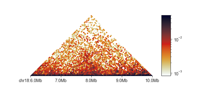
You can change the color scale from linear to log using -l:
fancplot chr18:6mb-10mb -p triangular -l -vmax 0.05 output/hic/binned/fanc_example_50kb.hic
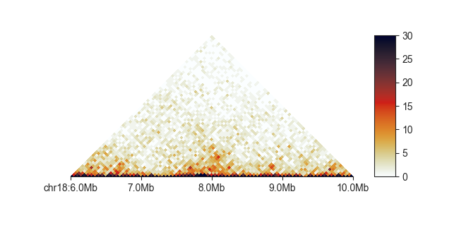
By default, triangular plots normalised matrix data. You can turn this off
on the fly to plot uncorrected data using -u:
fancplot chr18:6mb-10mb -p triangular -u -vmax 30 output/hic/binned/fanc_example_50kb.hic
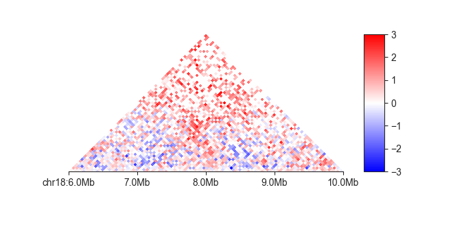
Similarly, you can convert the matrix on the fly to an observed/expected (O/E)
matrix using -e. When using this option, the matrix values are automatically
log-2 transformed and the colorscale adjusts to a divergent colormap symmetrical
around 0.
fancplot chr18:6mb-10mb -p triangular -e -vmin -3 -vmax 3 output/hic/binned/fanc_example_50kb.hic
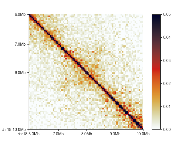
square
This plot is the common square matrix plot. It has nearly the same options as
triangle and uses the same syntax:
fancplot chr18:6mb-10mb -p square -vmax 0.05 output/hic/binned/fanc_example_50kb.hic
In addition to triangle, square supports flipping the matrix upside-down
with -f:
fancplot chr18:6mb-10mb -p square -f output/hic/binned/fanc_example_50kb.hic

split
The split plot divides a heatmap along the diagonal to compare two matrices.
split requires those matrices to be binned at the same resolution (or have identical
region definitions), as they are combined into a single merged matrix on the fly.
Besides providing two input matrices, one for the top and one for the bottom half
of the heatmap, the plot works in the same way as square.
The plot assumes that the matrices are directly comparable and have been normalised to
the same sequencing depth. If this is not the case, you can scale the matrices using
the -s parameter, but note that this could potentially take a very long time.
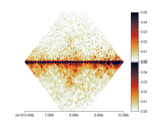
mirror
The mirror plot is built from two triangular heatmaps, the bottom one is flipped
upside-down to give the effect of a reflection along the horizontal axis. This can be
used to compare different matrices, including the same Hi-C dataset binned at different
resolutions:
fancplot chr18:6mb-10mb -p mirror -d 3mb output/hic/binned/fanc_example_50kb.hic output/hic/binned/fanc_example_100kb.hic
As this plot essentially consists of two triangular plots stapled together, the
parameters for the top and bottom plot can also be controlled independently. The
parameter names match those of the triangular plot, but with the u prefix
for the upper and l prefix for the lower plot:
--uvmin, --uvmax, --uc, --ue and
--lvmin, --lvmax, --lc, --le.
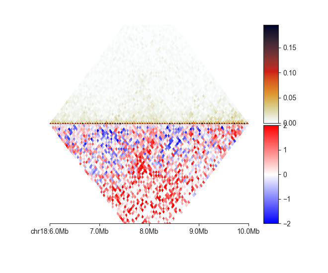
Here is one more example showing a matrix and its O/E transformed version:
fancplot chr18:6mb-10mb -p mirror -d 3mb -le -lvmin -2 -lvmax 2 output/hic/binned/fanc_example_50kb.hic output/hic/binned/fanc_example_50kb.hic