Basic usage¶

fancplot is modular and multiple plots can be combined into a single figure. Each plot can be configured individually, with a number of customisation options.

There are two modes: by default, an interactive plot opens in a new window, which allows synchronised scrolling, zooming and panning for plots that support it. By specifying an output file, the plot is saved to file directly.

Overview¶

fancplot plotting tool for fanc

usage: fancplot [<fancplot global parameters>] <region> [<region> ...]
            --plot <plot type> [<plot parameters>] <plot data file(s)> [...]

            Run fancplot --plot <plot type> -h for help on a specific subplot.

Plot types:

-- Matrix --
triangular    Triangular Hi-C plot
square        Square Hi-C plot
split         Matrix vs matrix plot
mirror        "Mirrored" matrix comparison plot

-- Region --
scores        Region scores plot with parameter dependency
line          Line plot
bar           Bar plot for region scores
layer         Layered feature plot
gene          Gene plot

Positional Arguments¶

regions

List of region selectors (<chr>:<start>-<end>) or files with region information (BED, GTF, …).

Named Arguments¶

`-o, --output`	Suppresses interactive plotting window and redirects plot to file. Specify path to file when plotting a single region, and path to a folder for plotting multiple regions.
`-s, --script`	Use a script file to define plot.
`-p, --plot`	New plot, type will be chosen automatically by file type, unless “-t” is provided.
`-n, --name`	Plot name to be used as prefix when plotting multiple regions. Is ignored for single region and interactive plot.
`--width`	Width of the figure in inches. Default: 4
`-w, --window-size`
	Plotting region size in base pairs. If provided, the actual size of the given region is ignored and instead a region <chromosome>:<region center - window size/2> - <region center + window size/2> will be plotted.
`--invert-x`	Invert x-axis for this plot
`--tick-locations`
	Manually define the locations of the tick labels on the genome axis.
`--verbose, -v`	Set verbosity level: Can be chained like “-vvv” to increase verbosity. Default is to show errors, warnings, and info messages (same as “-vv”). “-v” shows only errors and warnings, “-vvv” shows errors, warnings, info, and debug messages.
`--silent`	Do not print log messages to command line.
`-V, --version`	Print version information
`--pdf-text-as-font`
	When saving a plot to PDF, save text as a font instead of a path. This will increase the file size, sometimes by a lot, but it makes the text in plots editable in vector graphics programs such as Inkscape or Illustrator.

Setting up the figure and plotting regions¶

The main argument of fancplot is a region specification. You can list one or more regions by region selector (of the form <chromosome>:<start>-<end>), or you can provide the path to a file with region information (BED, GFF, FAN-C object, …). You can also mix the two. Regions will be plotted in the order they are listed with the next plot appearing after the previous one has been closed.

# single region
fancplot chr18:6mb-10mb

# multiple regions
fancplot chr18:12000000-14000000 chr18:6.5mb-10mb

# BED file
fancplot /path/to/file.bed

By default, fancplot plots exactly the area that is provided. It is, however, also possible to merely center the plot on the provided region, and to set a fixed plotting window using the -w option. This is especially useful when providing regions from other analyses, such as ChIP-seq peaks or insulation boundaries, and allows you to quickly survey other genomic features in their immediate surrounding.

fancplot -w 1mb /path/to/chipseq.narrowPeak

By default, fancplot will open an interactive plotting window. With the -o <path> argument, it is possible to directly plot to a file. The file ending determines its type.

fancplot -o /path/to/plot.png chr18:6mb-10mb

When specifying multiple regions, the output argument will be interpreted as a folder, and each plot will be named by the pattern <region index>_[<prefix>_]_<chromosome>_<start>_<end>. The <prefix> can be added using the --name argument.

The figure width is controlled using the --width argument (4 inches by default). The figure height is determined automatically from the figure width, the number of panels, and their aspect ratio.

Adding panels¶

After setting up the figure and plotting region(s), you can start adding plots to the figure. On the command line, the -p or --plot argument adds a new panel. You need to provide the type of plot you want immediately after -p:

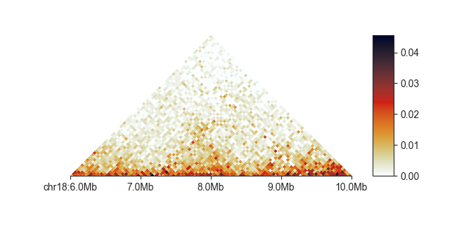
fancplot chr18:6mb-10mb -p triangular

A basic call to fancplot, plotting a 4 Megabase region on chromosome 18 of a Hi-C matrix in a triangular heatmap, could look like this:

fancplot chr18:6mb-10mb -p triangular output/hic/binned/fanc_example_50kb.hic

../_images/fancplot_triangular_example.png

fancplot tries to find a sensible placement of ticks and ticklabels on the genome axis, but if you prefer different tick locations or if labels are overlapping in small figures, define your own custom labels with the --tick-locations argument.

fancplot chr18:6mb-10mb --tick-locations 8mb 10mb -p triangular output/hic/binned/fanc_example_50kb.hic

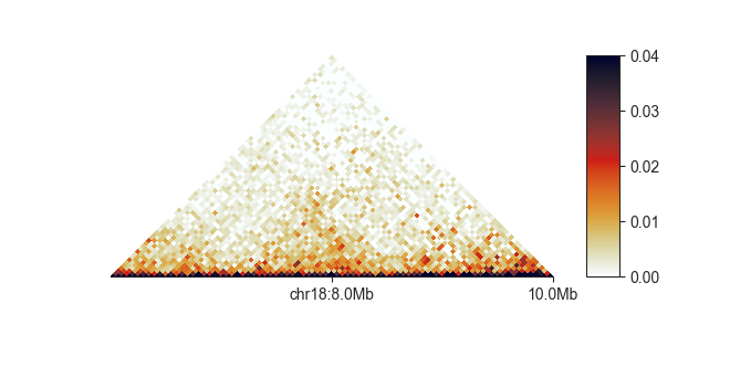
../_images/fancplot_triangular_example_custom_ticks.png

The first label will always get a chromosome prefix.

To get help on a specific panel type, and list available parameters, use -h after the plot type:

fancplot chr18:6mb-10mb -p triangular -h

Common parameters¶

A few parameters are supported by all panel types. For example, you can set a title above a panel using the --title parameter.

You can format the genome axis in various ways. For example, add minor ticks between the major ones on the genome axis using --show-minor-ticks, or hide the major ticks, too using --hide-major-ticks. You can add a small legend to the panel showing the distances between minor and major ticks, as well as the size of the plotting region with --show-tick-legend. You can hide the x axis altogether with --hide-x.

The aspect ratio of each plot controls the height of the y axis relative to the width of the x axis. For example, the default aspect ratio of the square plot is 1.0 while the default for triangular is automatically determined so that the matrix is not distorted.

Sometimes there might be a nomenclature mismatch in the data backing different panels regarding chromosome naming (with or without the chr prefix). Rather than having to reformat your data to match with the plotting region definition, you can correct for this issue on the fly, for each panel separately using --fix-chromosome.

In the following sections we will introduce the different Panel types in more detail.