Expected values¶

Note

The following examples use the matrix files in FAN-C format. If you want to try the first few commands using Juicer .hic files, replace output/hic/binned/fanc_example_500kb.hic with architecture/other-hic/fanc_example.juicer.hic@500kb. If you want to work with Cooler files in this tutorial, use architecture/other-hic/fanc_example.mcool@500kb. The results will be minimally different due to the “zooming” and balancing applied by each package.

The contact intensity in a Hi-C matrix gets progressively weaker the further apart two loci are. The expected values follow a distinctive profile with distance for Hi-C matrices, which can be approximated by a power law and forms an almost straight line in a log-log plot.

To calculate the expected values of any FAN-C compatible matrix, you can use the fanc expected command:

usage: fanc expected [-h] [-p PLOT_FILE] [-l LABELS [LABELS ...]]
                     [-c CHROMOSOME] [-tmp] [--recalculate] [-N]
                     input [input ...] output

Positional Arguments¶

`input`	Input matrix (Hi-C, fold-change map, …)
`output`	Output expected contacts (tsv).

Named Arguments¶

`-p, --plot`	Output file for distance decay plot (pdf).
`-l, --labels`	Labels for input objects.
`-c, --chromosome`
	Specific chromosome to calculate expected values for.
`-tmp, --work-in-tmp`
	Work in temporary directory
`--recalculate`	Recalculate expected values regardless of whether they are already stored in the matrix object.
`-N, --no-norm`	Calculate expected values on unnormalised data.

Example¶

The following example calculates and plots the expected values for a 500kb resolution Hi-C matrix of chromosome 19.

fanc expected -p architecture/expected/fanc_example_500kb_expected.png \
              -c chr19 \
              output/hic/binned/fanc_example_500kb.hic \
              architecture/expected/fanc_example_500kb_expected.txt

The resulting plot (from -p) looks like this:

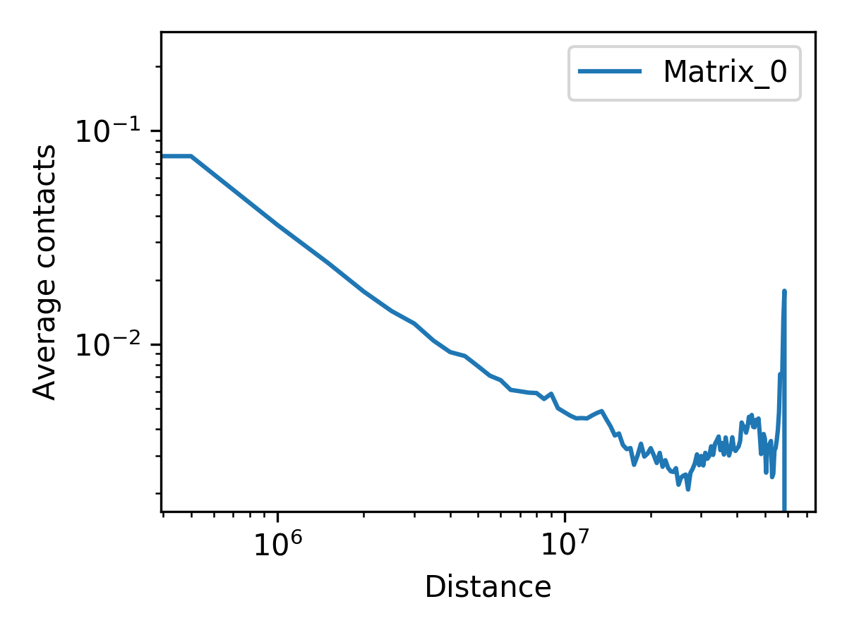
../../_images/fanc_example_500kb_expected.png

The actual expected values are stored in architecture/expected/fanc_example_500kb_expected.txt:

distance    Matrix_0
0   0.24442297400748084
500000      0.07759323503191953
1000000     0.03699383283713825
1500000     0.02452933204893787
2000000     0.017725227895561607
2500000     0.014272302693312262
3000000     0.011708011997703627
3500000     0.010125456912234796
...

Options¶

The expected values are stored in the matrix. If you are running any command that relies on the expected values again, it will be retrieved rather than recalculated. Use --recalculate to force a re-calculation of expected values, for whatever reason.

It may be interesting to plot the expected values of unnormalised matrices, to see any ranges where contacts are more or less abundant before normalisation. Use -N to plot the unnormalised expected values.

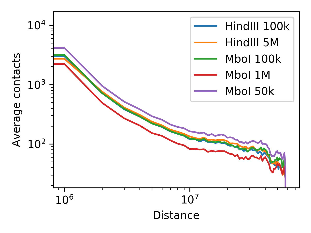
Comparing expected values¶

When you are providing more than one matrix as input to fanc expected, the expected values for all matrices will be written to file and plotted if using the -p option:

fanc expected -l "HindIII 100k" "HindIII 5M" "MboI 100k" "MboI 1M" "MboI 50k" \
              -c chr19 -p architecture/expected/expected_multi.png \
              architecture/other-hic/lowc_hindiii_100k_1mb.hic \
              architecture/other-hic/lowc_hindiii_5M_1mb.hic \
              architecture/other-hic/lowc_mboi_100k_1mb.hic \
              architecture/other-hic/lowc_mboi_1M_1mb.hic \
              architecture/other-hic/lowc_mboi_50k_1mb.hic \
              architecture/expected/expected_multi.txt

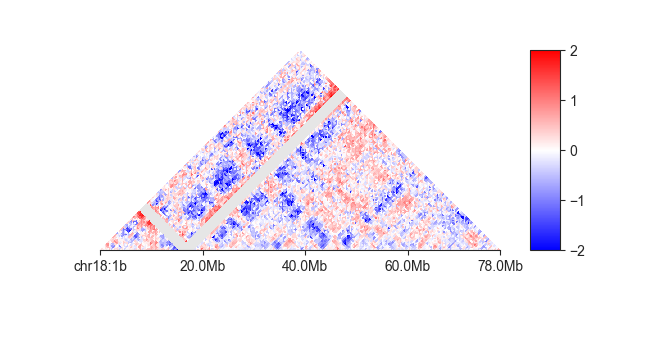
O/E matrices¶

Using fancplot, we can visualise the observed/expected Hi-C matrix, which normalised each matrix value to its given expected value at that distance. Here, we are showing a log2-transformed O/E matrix:

fancplot -o architecture/expected/fanc_example_500kb_chr18_oe.png \
     chr18:1-78mb -p triangular -e output/hic/binned/fanc_example_500kb.hic \
     -vmin -2 -vmax 2