AB compartment analysis

Note

The following examples use the matrix files in FAN-C format. If you want to try the same commands using Juicer .hic files, replace output/hic/binned/fanc_example_1mb.hic with architecture/other-hic/fanc_example.juicer.hic@1mb. If you want to work with Cooler files in this tutorial, use architecture/other-hic/fanc_example.mcool@1mb. The results will be minimally different due to the “zooming” and balancing applied by each package.

Regions in a Hi-C matrix can generally be assigned to either the active or the inactive compartment, also called ‘A’ and ‘B’ compartments, respectively.

usage: fanc compartments [-h] [-d DOMAINS] [-v EIGENVECTOR]
                         [-e ENRICHMENT_FILE] [-m MATRIX_FILE] [-g GENOME]
                         [-w] [-r REGION] [-i EIGENVECTOR_INDEX]
                         [-p PERCENTILES [PERCENTILES ...]] [-c COLORMAP]
                         [-s SYMMETRIC_AT] [--enrichment-min VMIN]
                         [--enrichment-max VMAX] [-G]
                         [-x EXCLUDE [EXCLUDE ...]]
                         [--compartment-strength COMPARTMENT_STRENGTH_FILE]
                         [-tmp] [-f] [--recalculate]
                         matrix [ab_compartments]

Positional Arguments

matrix	Input matrix (Hi-C, fold-change map, …) or existing AB compartment matrix.
ab_compartments
	AB compartment matrix file.

Named Arguments

-d, --domains	Write AB domains to this file. AB domains are output in BED format, and include the domains type (A/B) in the name field, and the eigenvector values (averaged across all bins in the domain) in the score field
-v, --eigenvector
	Write eigenvector values to this file.Output format is BED, containing of each matrix bin. The score field contains the eigenvector value of the bin.
-e, --enrichment-profile
	Plot AB enrichment profile to this file.
-m, --enrichment-matrix
	Path to save enrichment profile matrix (numpy txt format)
-g, --genome	Genome file. Used to “orient” the eigenvector values (change sign) using the average GC content of domains. Possible input files are FASTA, folder with FASTA, comma-separated list of FASTA) used to change sign of eigenvector based on GC content.
-w, --whole-genome
	Calculate AB compartments on the whole genome matrix, instead of individual chromosomes. Only enable if you are sure your use-case requires it. This is likely to introduce artefacts when working with matrices that have been normalised per-chromosome.
-r, --region	Only outputs domains / eigenvector values in this region. Only works with the -d and -e arguments. Compartmentalisation is always calculated on the whole genome.
-i, --eigenvector-index
	Eigenvector index. By default, the first eigenvector is output for eigenvector and domain analysis. Sometimes, it is useful to choose a higher eigenvector. E.g. for second eigenvector,specify “-i 2”.
-p, --enrichment-percentiles
	Percentiles to use for calculation of the enrichment profile. By default uses 20, 40, 60, 80, 100. The 0 percentile is included by default.
-c, --enrichment-colormap
	Matplotlib colormap to use for plotting the enrichment profile.
-s, --enrichment-symmetric-at
	Make enrichment profile plot symmetric around this value (e.g. use 0 to ensure that 0 is in the center of the plot).
--enrichment-min
	Minimum saturation value in enrichment profile. Default -1
--enrichment-max
	Maximum saturation value in enrichment profile. Default: 1
-G, --only-gc	Only use GC content for enrichment profile calculation, not the correlation matrix eigenvector.
-x, --enrichment-exclude
	Chromosome names to exclude from AB compartment and enrichment profile calculation
--compartment-strength
	File for saving the compartment strength as defined by Flyamer, Gassler, and Imakaev et. al (2017) (https://pubmed.ncbi.nlm.nih.gov/28355183).
-tmp, --work-in-tmp
	Work in temporary directory
-f, --force	Force overwriting of output files.
--recalculate	Force recalculation of eigenvector even if a vector with the same parameters has previously been calculated.

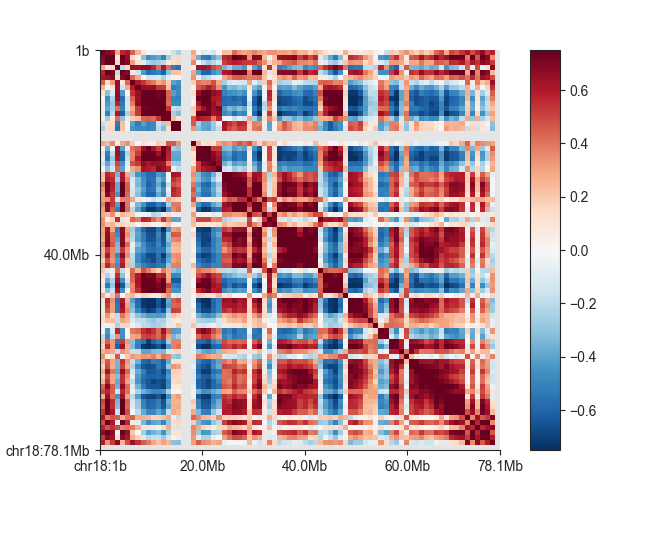
Correlation matrix

Compartments are derived from a correlation matrix, in which each entry i, j corresponds to the Pearson correlation between row i and column j of the (Hi-C) matrix.

The fanc compartments command can produce a correlation matrix (AB compartment) object from a FAN-C matrix file. Example:

fanc compartments output/hic/binned/fanc_example_1mb.hic architecture/compartments/fanc_example_1mb.ab

By default, compartment matrices are calculated on a per-chromosome basis, since each chromosome might be normalised differently. To force the AB calculation on the whole genome, use the -w option.

We can quickly plot the correlation matrix using the fancplot command:

fancplot -o architecture/compartments/fanc_example_1mb.ab.png chr18 \
     -p square architecture/compartments/fanc_example_1mb.ab \
     -vmin -0.75 -vmax 0.75 -c RdBu_r

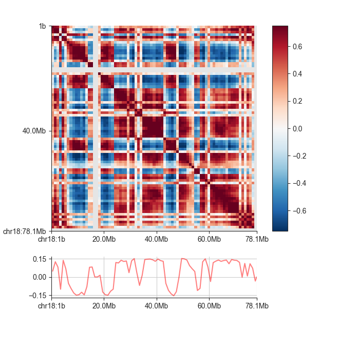
AB Eigenvector

The eigenvector of the correlation matrix is used to derive compartment type and strength for each matrix bin. Generally, regions with positive values are assigned the ‘A’, regions with negative values the ‘B’ compartment. To calculate the eigenvector in addition to the correlation matrix, simply add the -v <file_name> option to the previous command:

fanc compartments -v architecture/compartments/fanc_example_1mb.ev.txt \
                  output/hic/binned/fanc_example_1mb.hic \
                  architecture/compartments/fanc_example_1mb.ab

If architecture/compartments/fanc_example_1mb.ab already exists, it will not be recalculated but the matrix is loaded from file. You can use the -f option to overwrite the existing file in any case.

Alternatively, if you have already calculated the correlation matrix previously, simply run

fanc compartments -v architecture/compartments/fanc_example_1mb.ev.txt \
                  architecture/compartments/fanc_example_1mb.ab

Note that I have not specified an output file for the correlation matrix in this case.

We can plot the eigenvector using fancplot:

fancplot -o architecture/compartments/fanc_example_1mb.ab_and_ev.png chr18 \
     -p square architecture/compartments/fanc_example_1mb.ab \
     -vmin -0.75 -vmax 0.75 -c RdBu_r \
     -p line architecture/compartments/fanc_example_1mb.ev.txt

fanc compartments outputs the first eigenvector by default. In some cases it might be useful to choose a different eigenvector (sometimes the first eigenvector identifies chromosomal arms rather than compartments). To change the eiegnvector use the --i option, e.g. -i 2 for the second instead of the first correlation matrix eigenvector.

The sign of the eigenvector does not necessarily correspond well to the A or B compartment. Often, the eigenvector is “flipped” (inverted signs on its entries). Mathematically, if x is an eigenvector, so is -x. You can use external information to “orient” the eigenvector, so that it most likely corresponds to the active and inactive compartments. Specifically, you can supply a FASTA file with the genomic sequence to fanc compartments using the -g <fasta_file> argument. This is generally a good idea: fanc compartments then calculates the average GC content of regions with positive and those with negative eigenvector entries. As GC content has previously been shown to correlate well with compartmentalisation, the eigenvector is oriented in such a way that negative entries correspond to ‘B’ (low GC content) and positive entries to ‘A’ (high GC content).

fanc compartments -g hg19_chr18_19.fa -v architecture/compartments/fanc_example_1mb.ev_gc.txt \
                      architecture/compartments/fanc_example_1mb.ab

AB domains

Consecutive matrix bins with the same eigenvector sign are considered part of a “domain”. You can use the -d <domain_file> option to write the AB domains to a BED file:

fanc compartments -d architecture/compartments/fanc_example_1mb.domains.bed \
                      architecture/compartments/fanc_example_1mb.ab

Again, it is recommended to supply the genome for a better assignment of ‘A’ and ‘B’ to each domain:

fanc compartments -g hg19_chr18_19.fa \
                  -d architecture/compartments/fanc_example_1mb.domains_gc.bed \
                  architecture/compartments/fanc_example_1mb.ab

The domains BED file merges all consecutive bins in the same domain, which is why A and B are always alternating. It contains the domain type in the “name” field and the average eigenvector entry values of all bins in the domain in the “score” field:

chr18       1       3000000 B       -0.08663299058874448    .
chr18       3000001 4000000 A       0.09744158387184143     .
chr18       4000001 6000000 B       -0.1033548042178154     .
chr18       6000001 14000000        A       0.11616017390042543     .
chr18       14000001        16000000        B       -0.08352501317858696    .
chr18       16000001        24000000        A       0.08437945414334536     .
chr18       24000001        33000000        B       -0.10840386855933401    .
chr18       33000001        34000000        A       0.06491707265377045     .
chr18       34000001        43000000        B       -0.12647992662257618    .
chr18       43000001        49000000        A       0.09771443787030876     .
...

AB enrichment profiles

The compartmentalisation of a genome can be visualised in an enrichment profile plot. This will divide bins into percentiles using the associated eigenvector values, and then the average observed/expected (O/E) values of contacts in each pair of percentile bins is calculated and plotted.

Use the -e <plot_file> option to generate this plot. You can also use the -m <matrix_file> option to output the enrichment matrix values to file for further analysis.

fanc compartments -e architecture/compartments/fanc_example_1mb.ab_profile.png \
                  output/hic/binned/fanc_example_1mb.hic \
                  architecture/compartments/fanc_example_1mb.ab

Note that for the enrichment plot you will also need to provide the Hi-C matrix file for enrichment calculation. If the AB compartment matrix already exists at the output location, it will not be overwritten unless you are using the -f option.

As with the above commands, it is highly recommended to supply a genome file to properly orient the eigenvector:

fanc compartments -g hg19_chr18_19.fa \
                  -e architecture/compartments/fanc_example_1mb.ab_profile.png \
                  output/hic/binned/fanc_example_1mb.hic \
                  architecture/compartments/fanc_example_1mb.ab

This is what the plot looks like for the example:

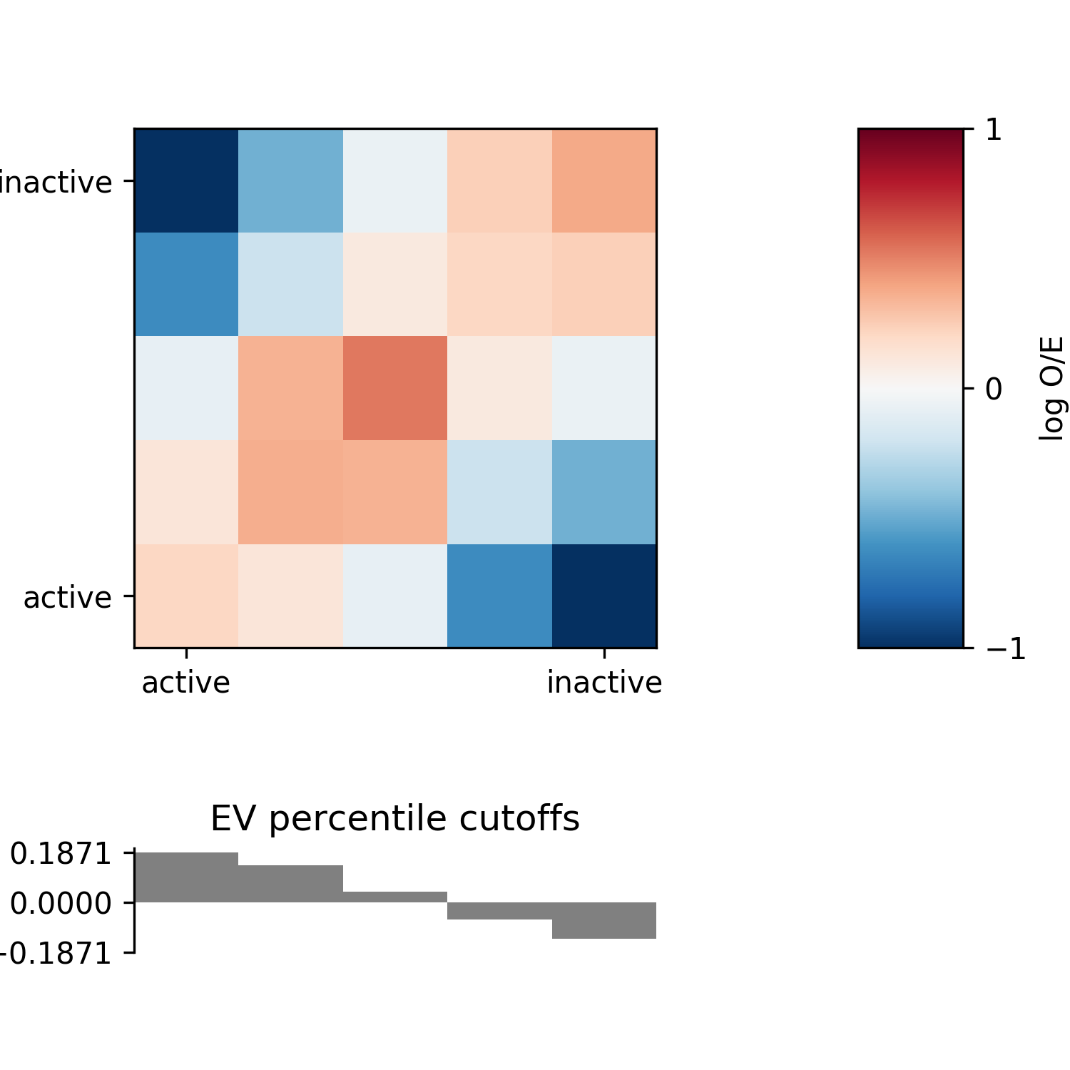
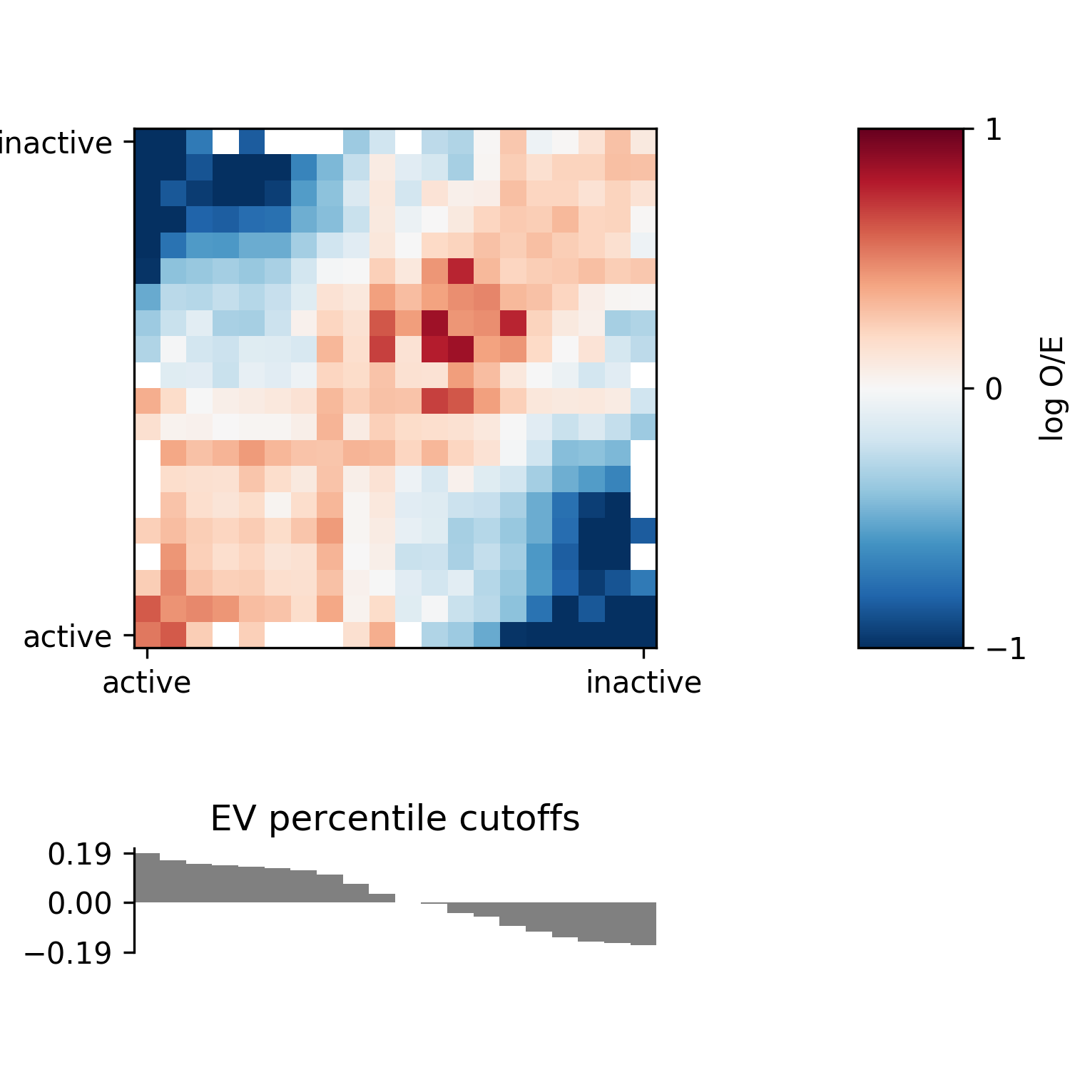
You can customise the enrichment analysis using additional parameters. By default, the percentiles for eigenvector binning are chosen at 20, 40, 60, 80, and 100. To choose a finer binning, for example, you can use -p 10 20 30 40 50 60 70 80 90 100. The “0” percentile is always added automatically. The eigenvector values are not necessarily centred around 0, which can lead to some unexpected enrichment plots. To force the central enrichment matrix bin to 0, and perform separate percentile calculations for values < 0 and >= 0, use the -s 0 option. Note, however, that this will lead to differences in the number of bins plotted on the left and right side of the matrix.

To format the plot, you can choose a different colormap with -c <cmap>. See here for colormap options. You can set the colorbar scale with --enrichment-min <n> and --enrichment-max <n>, where n is -1 and 1, respectively.

Compartment stength as defined by Flyamer, Gassler, and Imakaev et. al 2017 (https://pubmed.ncbi.nlm.nih.gov/28355183) can be calculated using --compartment-strength <filename>. It is defined in their supplement as follows “[In a 5x5 compartment enrichment map, ] “to calculate the strength of compartment signal, we took the natural logarithm of the AA * BB / AB^2”.